Understanding and Implementing Policy Gradients

Policy gradients are a pretty cool class of reinforcement learning algorithms. They focus on directly optimizing the metric we care most about in reinforcement learning (the expected reward from acting in an environment), and because of this enjoy an elegant formulation that looks very similar to supervised maching learning, and has stability benefits over approaches like Q-learning, which indirectly learn a policy, and can suffer from too much approximation.

While this blog post is in no sense comprehensive, I hope to show a good mixture of theory and practice. There’s a lot of great blog posts out there on policy gradients and/or deep reinforcement learning, and many go into depth in the mathematical fundamentals or empirical observations. I hope to provide a pedagogically useful blogpost that introduces the concepts, derivations, python implementation examples, and empirical observations that help us go from simple Vanilla Policy Gradient, to the more advanced Trust Region Policy Optimization, and then to Proximal Policy Optimization, which is conceptually similar to TRPO but much easier to implement (and thus a popular sota baseline.)

Credits go to Daniel Takeshi’s blog, John Schulman’s PhD thesis, OpenAI’s Spinning Up, and the Stanford CS234 lectures, from which the explanations in this post are synthesized.

Vanilla Policy Gradient

Let’s first implement vanilla policy gradient (REINFORCE), the backbone of these three methods. (My acknowledgements go to Daniel Takeshi, since this section is highly based off of his blog post.)

The goal of reinforcement learning is for an agent to learn to act in a dynamic environment so as to maximize its expected cumulative reward over the course of a time-horizon. Policy gradient methods solve the problem of control by directly learning the policy \(\pi: \mathcal{S} \rightarrow \mathcal{A}\) from observations of rewards obtained by interacting with the environment.

Formally define a trajectory \(\tau\) as a tuple \((s_0, a_0, r_0, s_1, a_1, ..., r_T)\) denoting a sequence of state-action-rewards observed over the course of some episode of interaction with the agent’s environment, and let \(R(\tau)\) denote the finite-horizon return, aka cumulative sum of rewards over finite timesteps. Then our goal is the maximize the expected finite-horizon return where the expectation is over trajectories sampled from the stochastic policy \(\pi_{\theta}\) (here we let \(\theta\) denote the parameters of the policy \(\pi\))–i.e.

In order to optimize \(J\) using gradient ascent, we need an efficiently computable form of its gradient. First, let’s compute an analytical form of the gradient, then see how we can approximate it with sampling.

We use the log-derivative trick to push a form of the gradient of the policy into the the gradient of \(J\).

I liked Daniel Takeshi’s explanation of it–“the log derivative trick tells us how to insert a log into an expectation when starting from \(\nabla_{\theta} \mathbb{E}[f(x)]\)”

In the gradient of \(J\) we are concerned with the gradient of the log probability of trajectories, so we derive its form now.

Note that the dynamics of the environment \(P\) disappears, as it does not depend on \(\theta\), which shows that policy gradients can be used in a model-free manner.

Putting the pieces together, the gradient of the expected return is

The log probability of each action is weighted by the rewards associated with it. The gradient has an intuitive interpretation–it encourages us to increase the probability of actions which lead to high expected return.

Conveniently, \(\nabla_{\theta} J\) turns out to have the form of an expectation. Because of this, as long as we can take the gradient of the log of our policy, we can estimate it with Monte Carlo simulation using samples from our environment–i.e.

Where \(\mathcal{D}\) is a dataset of trajectories.

Policy Network

The policy is represented as a multi-layer perceptron, since we are interested in acting in high dimensional state spaces with continuous actions. (On an aside, a less utilitarian and very beautiful thing about deep RL is that it connects neuroscience with artificial intelligence. Here’s recent work on connections between TD-learning and dopamine in animal learning.)

def build_mlp(input_size, output_size, n_layers, size):    
    modules = OrderedDict()
    modules['Linear_Input'] = nn.Linear(input_size, size)
    modules['ReLU_Input'] = nn.ReLU()
    for i in range(n_layers):
        modules['Linear_'+str(i)] = nn.Linear(size, size)
        modules['ReLU_'+str(i)] = nn.ReLU()
    modules['Linear_Output'] = nn.Linear(size,output_size)
    sequential = nn.Sequential(modules)
    return sequential

policy_network = build_mlp(observation_dim, 1, n_layers, layer_size)

Below is the implementation of the policy gradient update. Note here that advantage denotes \(\sum_{t' = t}^T r_{t'}- V^{\pi}(s_t)\)

def update_policy(self, observations, actions, advantages):

        self.optimizer.zero_grad()
        res = self.policy.action_distribution(observations).log_prob(actions) 

        loss = -(res * advantages).mean()
        loss.backward()
        self.optimizer.step()

Variance

An issue with the estimator \(\hat{g}\) is that it has high variance. One of the reasons for this is that \(R(\tau)\) sums up individual reward samples over long sequences.

To see this, let \(R_t = \sum_{i=0}^t r_t\), the sum of rewards up to time step \(t\). Then in general, a longer trajectory has a higher variance in cumulative rewards than a shorter trajectory, since rewards are correlated within an episode. (Intuitively, the actions you take influence the distribution of future states you will see, and also the actions further available to you.) To formally see this,

(as long as \(\sum_{i=0}^t Cov(r_i, r_{t+1})\) is non-negative.)

If we have high variance in our estimate of the policy gradient, then the update will cause the policy to fluctuate across updates.

Variance Reduction 1: Rewards-To-Go

One way to decrease variance of the estimator starts by observing that the action taken at time \(t\) affects only the rewards reaped at timestep \(t\) onwards. This makes sense in terms of credit assignment, and also reduces the number of timesteps we sum over. Let’s do some algebra to get the gradient into a form we want:

The literature likes to refer to \(\sum_{t' = t}^T r_{t'}\) as rewards-to-go. We weight each action by its causal consequence–the future rewards it impacts.

Variance Reduction 2: Baseline

A second way to decrease the variance of the policy gradient estimate is by subtracting a baseline from the rewards-to-go.

An intuitive choice for \(b(s_t)\) is the state-value function \(V^{\pi}(s_t)\). When we use the state-value function as a baseline, we are choosing to weight an action by the difference between the rewards we got in our sample and the rewards we expected to get. If the difference is close to zero, then we shouldn’t need to change our policy too much–i.e. the gradient for that state-action should be close to zero in the update.

To more formally explain why the baseline reduces the variance of the policy gradient estimator, I’ll summarize Daniel Takeshi’s explanation, which is an approximate one.

He first approximates the variance of a sum by the sum over timesteps of variances. Then he uses the formula \(Var(X) = \mathbb{E}[X^2] - (\mathbb{E}[X])^2\) noting that \(\mathbb{E}[X] = 0\) for the log probability form. The third approximation comes from independence. Daniel Takeshi says that the approximations are fine since recent advances in RL, like A3C, break up correlation among samples.

Based on these approximations, we can see that that a well-chosen baseline can decrease the variance of \(\hat{g}\).

Baseline Refitting

Note that we will have to update the baseline, \(V^{\pi}(s_t)\) every time we perform a policy update. This is because we want our estimate of the value function to be as accurate as possible, given the data we have. To do so, we compute the mean squared error loss between a forward pass of the network (current value estimate) and the most recent returns we have.

def update_baseline(self, returns, observations):
        
        self.optimizer.zero_grad()
        preds = self.forward(observations)
        loss = ((returns - preds)**2).mean()
        loss.backward()
        self.optimizer.step()

Experiment

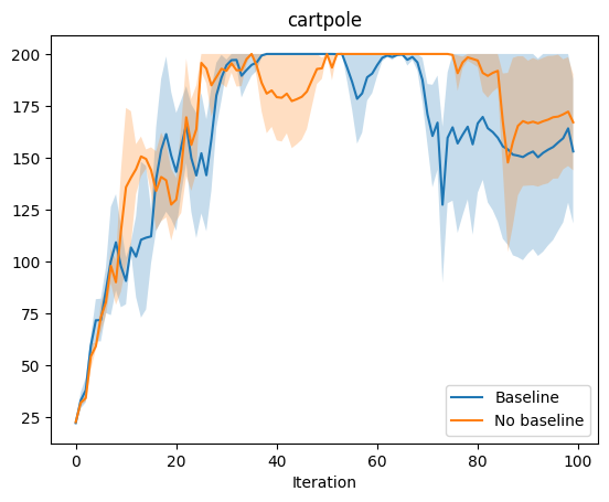
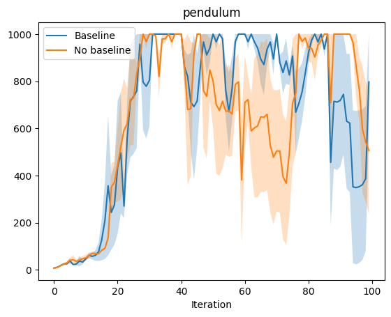
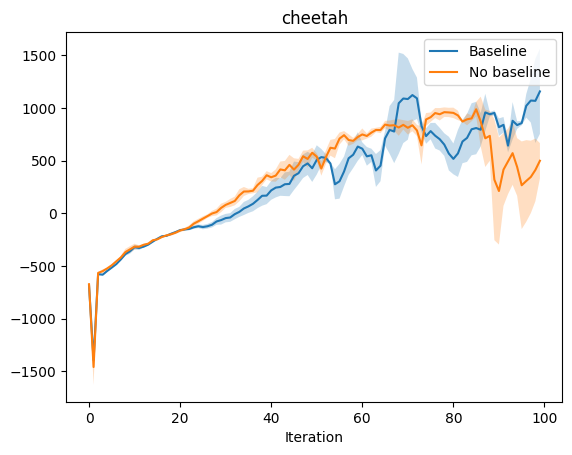
Now we are ready to run some experiments. We would hope to see that the introduction of the baseline improves performance over just using the returns in the policy gradient estimate. To do so, we experiment on three OpenAI gym environments–cartpole, pendulum, and half-cheetah. For each environment we choose three random seeds, and run the agent with and without baseline using those three seeds. We plot the average expected return for each experiment with error bars.

The cartpole and pendulum results do not really demonstrate the difference between baseline and no baseline, but cheetah seems to be a complex enough environment to show the difference. In cheetah, we see that the baseline approach outperforms no baseline, especially at the very end, where the no baseline approach actual deteriorates in performance while the baseline approach continues to improve. Without a baseline, the policy gradient updates may be too large. In fact, even with a baseline, VPG is too “greedy” an approach. An intuitive explanation is that overcorrecting (changing the way you act too drastically) based on feedback may incur immediate benefits but prevent long term learning and generalization. TRPO and PPO aim to make monotonic improvements in performance by constraining the difference between the policy before and after updates using KL-Divergence.

Empirical Results: Baseline vs no Baseline

Variance Reduction 3: TD Error

We do not implement this variant in this blog post, but another way to reduce variance, at the risk of adding bias, is by using Temporal Difference methods rather than Monte Carlo methods to estimate the policy gradient.

\(\sum_{t' = t}^T r_{t'} - V^{\pi}(s_t)\) is an estimate of a quantity we call the advantage, \(A^{\pi}(s_t,a_t)\). This formulation characterizes how much better our action was at time \(t\) in a given episode, over following some policy \(\pi\). Given this terminology, we are technically also optimizing

The advantage function is formally defined as

Instead of summing up over all future rewards in an episode, TD uses the reward at time step \(t\) as well as the current estimate of \(V\) to estimate the advantage. This is called bootstrapping, in contrast with the entire roll-outs or simulations that Monte Carlo performs

Let \(\delta_{t}^{\hat{V}} = r_t + \gamma \hat{V}(s_{t+1}) - \hat{V}(s_{t})\). Then if \(\hat{V} = V^{\pi}\), \(\delta_{t}^{\hat{V}}\) is an unbiased estimator of \(A^{\pi}\). However, in practice, \(\hat{V}\) is an imperfect estimate of \(V^{\pi}\) and \(\delta_{t}^{\hat{V}}\) ends up being biased because of it.

We can actually interpolate between TD and MC by controlling the number of time steps we sum rewards over before using the bootstrapped estimate of future rewards. Define

Then after cancelling out some telescoping sums,

Note that setting \(k = T\) pretty much gives us the original Monte Carlo estimate. As we showed above, summing over rewards for more time steps generally increases variance, and this form of TD / MC interpolation allows us to control somewhat how much variance tolerate.

Monotonic Improvement and TRPO

(My acknowledgements go to John Schulman, since this section is highly based off of his PhD thesis.)

As shown in the experiment above, VPG does not necessarily make monotonic improvements to the expected performance of a policy. TRPO constrains the step-size of the gradient updates to impose monotonic improvement. First we derive the theoretical basis for TRPO, then we look into the details and make approximations and estimates in order to implement it.

Instead of setting the optimization objective to be the expected performance of a policy, we instead set the objective to be a loss function whose monotonic improvement guarantees monotonic improvement of the policy itself. Consider the following identity due to Kakade and Langford,

Where \(\eta_{\pi}(\pi)\) is the discounted sum of rewards from following \(\pi\) and \(A_{\pi}(s_{t}, a_{t})\) is the advantage of taking action \(a_{t}\) over following \(\pi\) at time step \(t\). If we massage this equation into a slightly different form, we can begin to see the theoretical basis for TRPO.

If we define \(P(s_t = s \vert \tilde{\pi})\) to be the probability that we end up in state \(s\) at time \(t\) by following \(\pi\), then we can conveniently rewrite \(\eta_{\pi}(\tilde{\pi})\) as

Where \(p_{\tilde{\pi}}(s) = P(s_0 = s \vert \tilde{\pi}) + \gamma \cdot P(s_1 = s \vert \tilde{\pi}) + ...\) is the discounted state visitation frequency. From the formulation above, we can see that any policy update that has positive expected advantage at every state is guaranteed to improve policy performance.

However, in our computation of the policy update, we cannot compute \(p_{\tilde{\pi}}(s)\) as we do not have samples from the new policy \(\tilde{\pi}\). We make a local approximation to \(\eta\) by using \(p_{\pi}(s)\) instead, yielding the modified objective

The first order gradient of \(L_{\pi}(\tilde{\pi})\) and \(\eta_{\pi}(\tilde{\pi})\) are equivalent, which means we can indirectly improve \(\eta_{\pi}(\tilde{\pi})\) by directly optimizing \(L_{\pi}(\tilde{\pi})\). However, we do not yet know how large a step size we can take and still have guaranteed improvement.

A theorem from Kakade and Langford gives

Since \((D_{TV})^2\) is upper bounded by KL divergence, we also get

To see that we can get monotonic improvement by optimizing \(L\),

Let \(M_i(\pi) = L_{\pi_i}(\pi) - \dfrac{4 \epsilon \gamma}{(1-\gamma)^2} D_{KL}^{max}(\pi_{old}, \pi_{new})\)

Note that \(M_i(\pi_i) = L_{\pi_i}(\pi_i) = V^{\pi_i}\)

Then

\(\begin{align*} V^{\pi_{i+1}} & \ge L_{\pi_{i}}(\pi_{i+1}) - \dfrac{2 \epsilon \gamma}{(1-\gamma)^2} D_{KL}^{max}(\pi_{i}, \pi_{i+1}) \\ \end{align*}\) And subtracting \(V^{\pi_{i}}\) from both sides \(\begin{align*} V^{\pi_{i+1}} - V^{\pi_{i}} & \ge M_{i}(\pi_{i+1}) - M_{i}(\pi_{i})\\ \end{align*}\)

Since \(M_i(\pi_i) = V^{\pi_i}\).

Instead of optimizing \(M\), which includes a penalty term for the KL divergence, TRPO optimizes against a constraint on the KL divergence. There are sample-based ways to estimate the objective and constraint, which you can read about in John’s PhD thesis.

PPO

Since TRPO uses conjugate gradient descent to optimize the objective, we turn our focus on a simpler but similar algorithm, PPO. PPO is still motivated by the question of making monotonic improvements to a policy, but uses numerical methods which compute only first derivatives.

Here, we focus on PPO-Clip, which replaces the KL-divergence term by clipping the objective function to remove incentives to make big changes to the policy.

The PPO objective function is

where

where

We can view the clipping term as analogous to KL-constraining the old and new policies in TRPO. Taking the of min the clipped objective and unclipped objective corresponds to taking a pessimistic (i.e. lower) bound on the original object. In our implementation of PPO-clip, we set \(\epsilon=0.2\), which was shown in the PPO paper to lead to the best average performance.

Taking ratio of the old and the new log probabilities, in addition to being a way to measure the magnitude of policy change accross the update, serves another purpose. Notice that in the objective we are estimating the value for the policy with parameters \(\theta_{k+1}\) but our state-action samples are collected from the policy with parameter \(\theta_{k}\). Using \(\dfrac{\pi_{\theta}(a \vert s)}{\pi_{\theta_{k}(a \vert s)}\) allows us to re-weight our samples so we approximate the expectation of the loss with respect to \(\theta_{k+1}\). This common technique in RL is called importance sampling.

Here’s a snippet of the PPO update–

def update_policy(self, observations, actions, advantages, prev_logprobs):

        self.optimizer.zero_grad()
        res = self.policy.action_distribution(observations).log_prob(actions) 
        ratio = torch.div(res,prev_logprobs) 
        clipped_ratio = torch.clamp(ratio, 1-self.epsilon_clip, 1+self.epsilon_clip)
        loss = -(torch.min(ratio,clipped_ratio) * advantages).mean()
        loss.backward()
        self.optimizer.step()

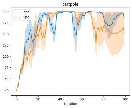
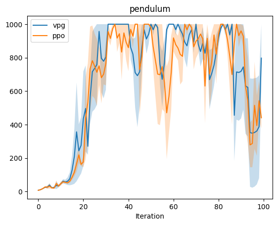
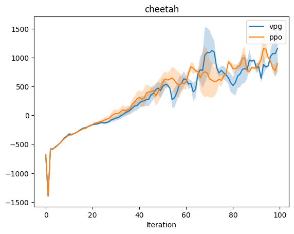
Experiment: PP0 vs VPG

The experiment in cartpole most clearly shows the advantages of PPO over VPG, espectially near the end of the experiment. One hypothesis for why PPO’s performance decays near the end is that the large steps in the updates could have caused settling on local optima. (Viewing videos of the training performance could help one observe any high-level behaviors that emerge.) As with the case in the VPG baseline / no-baseline experiments, there’s a bit too much noise in the pendulum environment to draw conclusions. In the cheetah environment, PPO initially outperforms VPG, though near the end, both are brittle. Note that the performance we observe for PPO is not strictly monotonic. The clipped objective does constrain the size of updates, though there are no formal guarantees in the style of the TRPO guarantee. Work on PPO addresses this issue in a number of ways, including early stopping. It is also worthy to note that policy gradients are sensitive to batch size, advantage normalization, and policy architecture.